Introduction
This describes a Visual Basic program which calculates and displays graphically information on the planets and their major satellites. Its aim is primarily to help amateur astronomers understand and see Mars, Jupiter, and Saturn and the phenomena associated with their satellites. ( I am not sure if the Visual Basic program can be accessed by the user . I am working on this and further modifications need to be done, especially towards showing and running the source code. ???)
It is not the sort of program that can be written in a week, or a month, or ……., as will be seen in the descriptions below. Major steps in the program are to calculate:
- At the chosen time, the heliocentric positions ( relative to the Sun) of the Earth and the planets.
- The geocentric positions (relative to the Earth) of the planets – Right Ascension and Declination.
- For a chosen position of Latitude and Longitude on Earth, the Hour angle, azimuth and altitude.
( Of course, any number of software programs are available to do the above. Here, it is necessary to do these calculations for what follows and they need to be done with high accuracy.) - Planetary information such as Visual magnitude, apparent inclination of the equator to the ecliptic, apparent angular diameter, phase, apparent shape, longitude of central meridian due to rotation, and also:
For Mars: Approximate extent of the polar caps;
For Jupiter: Position of the Great Red Spot, the appearance of the belts;
For Saturn: Appearance of bands on the planet and the appearance of the rings;
Declination of the Sun and the Earth as seen from the ring plane (this is used to determine the openness of the rings as seen and possible invisibility of the rings); Increase in brightness caused by the rings; Position of shadow of ring on the planet and of planet on the rings. - The positions of the major satellites of Mars, Jupiter, and Saturn in their orbits around the planet as seen from the Sun and from the Earth.
- Satellite phenomena such as transit, occultation, eclipse, and throwing shadows on the planet, as seen from Earth. These phenomena are common for the Jovian satellites (and fascinating) but rare for those of Saturn because of the high inclination of their orbits to the ecliptic.
- Mutual satellite phenomena (occultations and eclipses). These are relatively rare but even more special to see than the phenomena involving the satellite and Jupiter itself.
- The main graphical displays are then given to help the user understand what can be seen at the telescope. First, a plan view of the planet and satellite system ( looking down from above the plane of the solar system) with an indication of the direction of Earth and the shadow thrown by the Sun is displayed.
- Then the planet and the satellite system as seen through the telescope are displayed. This includes planetary features discussed above and the positions and visual magnitudes of the satellites. Eclipses, shadows and transits are shown. This is useful for the Jovian system in particular (but it has been used to predict and see eclipses and shadows of Titan). Satellites are not shown when occulted, shown as very dark ( to give an idea of the progress of the eclipse) when eclipsed, and shadows of the satellites are shown in the correct position on the planet. The orbit of the satellite is shown to further assist in showing the progress of the satellite.
This graphical data is accompanied by numerical data concerning the particular phenomenon. - Mutual satellite phenomena are reported and the size of the eclipsing shadow is shown relative to the size and position of the eclipsed satellite.
It can be seen that the main feature of the program concerns graphical display of the satellites and so it is called SatGraph for future reference.
NOTE:
I have recently downloaded the astronomical software program called STELLARIUM and began to make use of it.
I have found it to be very impressive and to give excellent views of the planets and their satellites. I hope that Satgraph does not just merely duplicate a portion of it but contains some additional calculations which may be useful to the amateur astronomer.
My hope is that Stellarium and Satgraph can complement each other in the areas that Satgraph concentrates on.
Also, I have recently changed Satgraph to use the data in the full VSOP87 theory. More details on this will be given shortly. The main change for the user is that the file PlanetPerturbII.txt is no longer needed but is replaced by 8 files VSOP87D.xxx.txt where xxx is Mer, Ven, Ear, Mar, Jup, Sat, Ura, and Nep.
The changes to the program alter the screenshots shown below slightly. I will work on bringing them up to date shortly.
Following Sections
Firstly, a User’s Guide to SatGraph is given so that amateur astronomers may hopefully use and benefit from SatGraph.
Then there is a section on Accessing and Using SatGraph.
Then, several Examples of its use are given.
For those interested in the Visual Basic programming, the program is described in a separate site “Programming and Technical Aspects” and for those wishing to understand the mathematics or to criticize the mathematics which I have done (welcome if it informs me or improves SatGraph), extensive explanation and references are also given in this site (of course, the programming and the technical details of the calculations are intimately connected). Link to Programming
Several other references may be given, but the main ones I have used are:
Astronomical Formulae for Calculators (2nd edition, 1982) by Jean Meeus (referred to as MeeusI)
Astronomical Algorithms (1st edition, 1991) by Jean Meeus (referred to as MeeusII)
Explanatory Supplement to the Astronomical Almanac, London, HM Stationery Office 1961 (referred to as ESI )
Explanatory Supplement to the Astronomical Almanac, Edited by P. Kenneth Seidelmann, Paperback impression 2006 first published 1992 (referred to as ESII)
User’s Guide to SatGraph
Several files are read by the program. These will be discussed in the section “Accessing and Using SatGraph” below. These files need to accompany the VB.Net code.
Note that the first two numbers in the planet file, Plan2000II.dtf, are the longitude and latitude of the observing site and should be changed by the user so that the program calculates the correct azimuth and altitude of the chosen planet at the specified time.
The longitude is positive for East and the latitude is positive for North and negative for South.
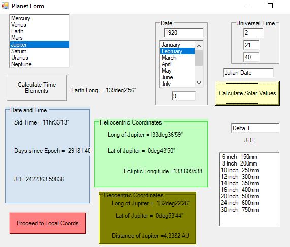
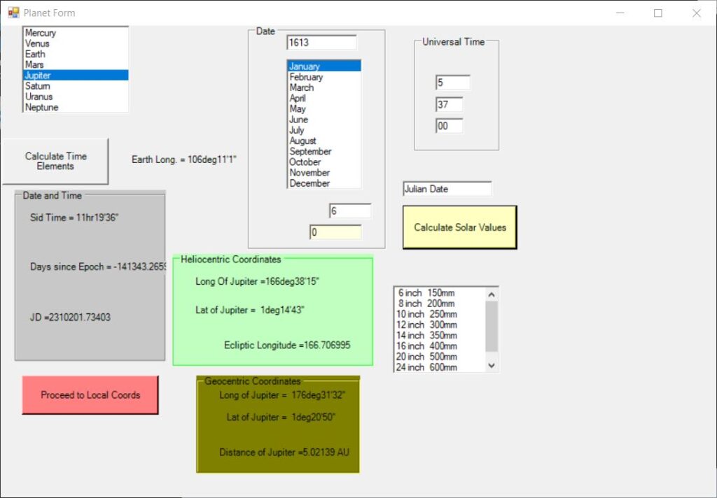
Main Form
When the main form comes up, the user needs to enter several pieces of data:
. The planet to be used is selected from a list.
. The date and time can be entered in two different ways.
Normally, one will enter the year, month, and day. The month is selected from a list but the year and day of the month need to be typed in. The time to be entered is Universal Time (Greenwich Mean Time) in hours, minutes, and seconds. The minutes and seconds are preset to zero and can be left at that if desired, but the hour needs to be typed in.
The Tab order is such as to make the above easier.
The other way is to enter the Julian Date, in which case the other entries are unnecessary. This is useful for checking results in the literature and may also be quicker for a clued-up observer.
. Delta T (the number of seconds between dynamic time and Universal time) can be entered. If it is not entered, it will be estimated by the program.
It is then necessary to click a button called Calculate Time Elements. It will then display the Sidereal time, the number of days elapsed since JD 2000.0, and the Julian Date.
The user should then click the button Calculate Solar Values.
The program will then display, in a group of Heliocentric coordinates for the chosen planet: Longitude; Latitude; and Ecliptic Longitude.
Then in a group of Geocentric Coordinates: Longitude; Latitude; and Distance, in Astronomical Units.
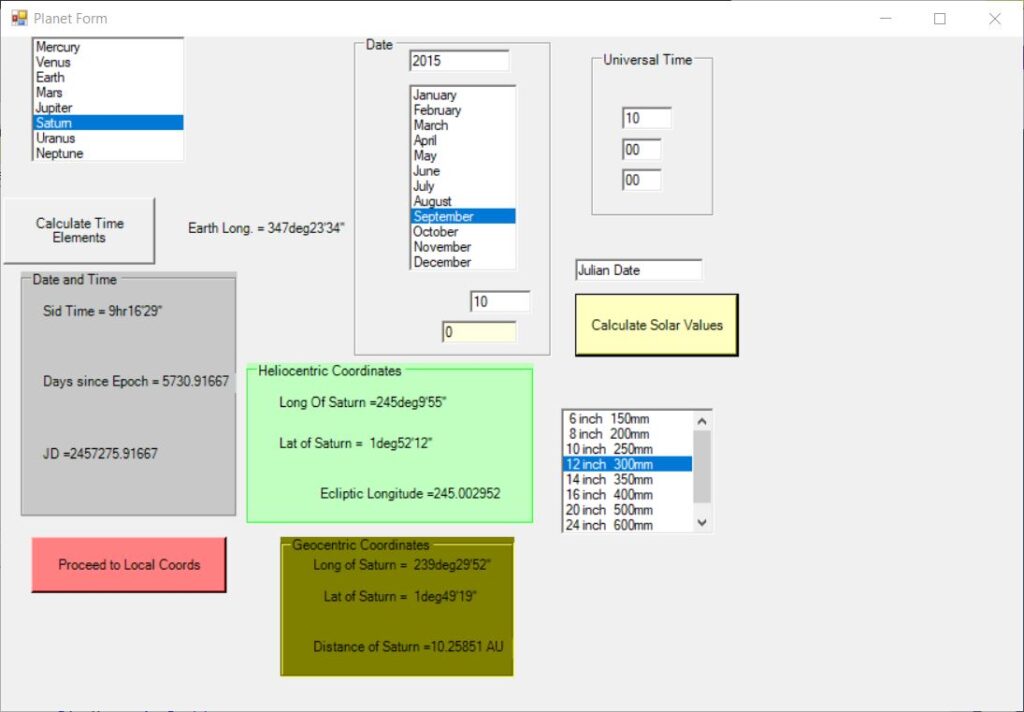
One then clicks the button “Proceed to Local Coords”.
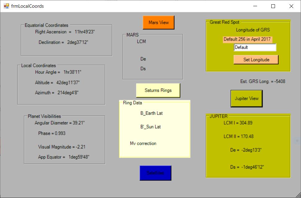
Local Coordinates form
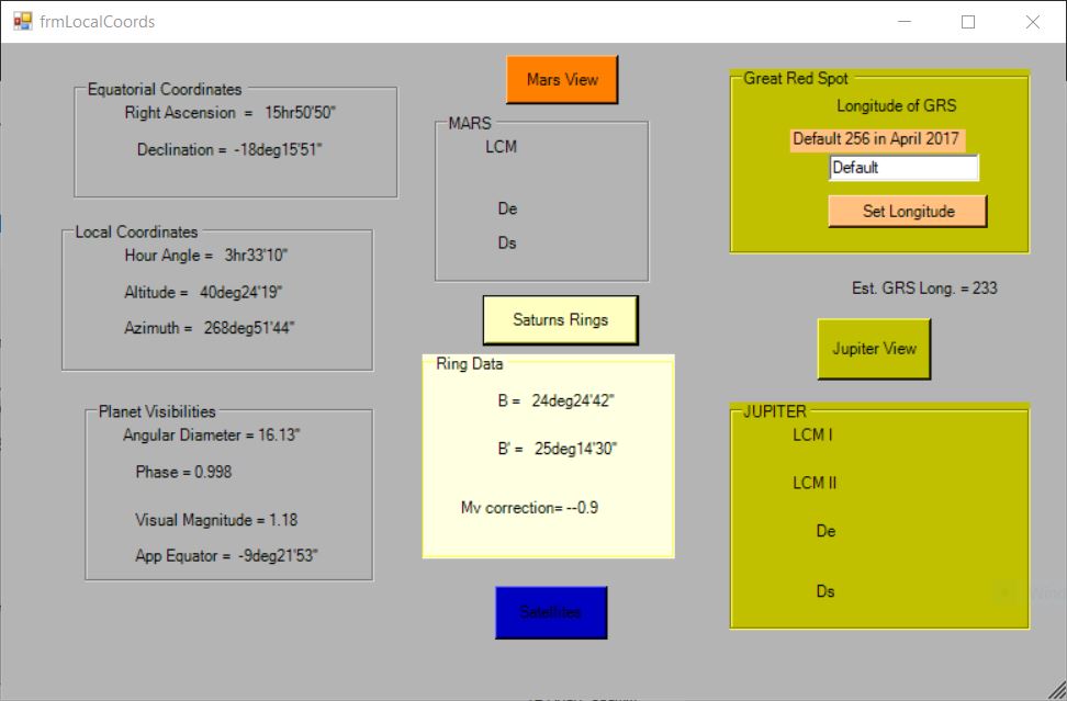
This is designed to show the position of the planet as seen by the observer and the appearance of the planet.
The positions shown are, in groups of Equatorial coordinates:
Right Ascension; and Declination.
Then in a group of Local coordinates:
Hour Angle; Altitude; and Azimuth. (These depend on the observer’s geographical position.)
In the group Planet Visibilities are displayed:
Angular diameter; Phase; Visual Magnitude; and apparent angle of equator to the Ecliptic.
Obtaining information about Mars or Jupiter, or Saturn’s rings, is optional by clicking buttons. However, if it is desired to have the position of the Great Red Spot subsequently displayed in the graphical part of the program, the “Jupiter View” button must be clicked.
This button will cause the display of: De; Ds; Longitude of Central Meridian (LCM) of System I; and LCM of System II. (De is the planetocentric ( as seen from Jupiter ) declination of the Earth, and Ds is the planetocentric declination of the Sun. It is possible to set the longitude of the GRS and this is probably necessary, rather than using the default value, as the longitude varies considerably.
Similarly, clicking “Mars View” will display:
De; Ds; and LCM for Mars.
Clicking Saturn’s Rings will display:
B (the Saturnicentric Latitude of the Earth, referred to the plane of the ring);
B’ (the same for the Sun); and the Visual magnitude correction due to the ring. This last will, of course, vary depending on whether the rings are relatively open or closed.
B and B’ will indicate relatively how open the rings are and, importantly, whether the rings are invisible due to the Earth looking at the unlit side. The rings are invisible if B and B’ are of opposite sign.
The user can then obtain information about the satellite system.
To proceed, click the “Satellites” button.
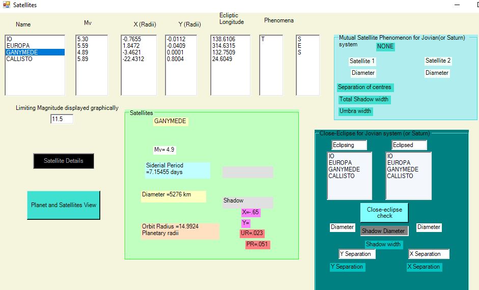
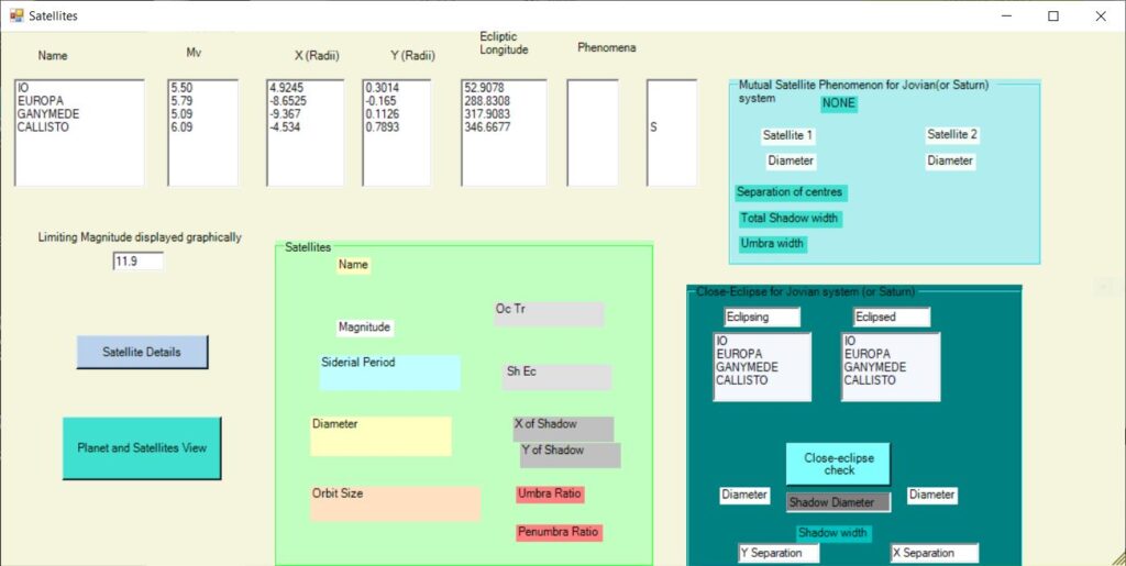
Satellites form
This will display data about the 4 major moons for Jupiter, or Phobos and Deimos for Mars, or Mimas, Enceladus, Tethys, Dione, Rhea, Titan, Hyperion, and Iapetus for Saturn.
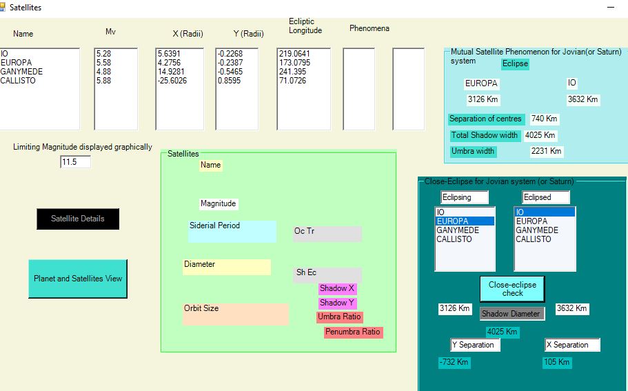
Here is shown the sample screen for the current Saturn example. Screens for Jupiter, which include additional data, are given below.

For each, it shows the apparent X and Y positions from the centre of the planet on the Ecliptic, in planetary radii. It also shows the Ecliptic longitude of the satellite with respect to the planet and any phenomena (Transit, Occultation, Eclipse in the shadow of the planet, or throwing a shadow onto the planet) that are occurring.
The phenomenon is deemed to start or end when the centre of the satellite is on the edge of the planet (or on the umbra of the shadow in the case of an eclipse). Information about position and time of starting and ending of phenomena is not shown here but can be obtained in the graphics form Telescope View (see below).
Note that in the screen above only Tethys, Dione, Rhea, and Titan are considered bright enough to see with this aperture (limiting magnitude 11.5).
It is possible to select a satellite in the list and click on “Satellite Details” button.
This will display the visual magnitude, the sidereal period in days, the diameter (in kilometers) and the orbital radius, in planetary radii.
It will also display whether it is currently involved in Occultation, Transit, Eclipse, or Shadow. If it is throwing a shadow, it displays the X and Y position of the shadow on the planet and the Umbra Ratio (UR= ) and Penumbra Ratio (PR=), where these are the ratios of the diameter of the shadow (in latitude on the planet since it may be foreshortened in longitude) to the diameter of the planet. An example and screen for Jovian satellites is given below.
It is also possible that one satellite will pass in front of another (occultation) or its shadow will pass across it (eclipse). These are called mutual satellite phenomena.
Mutual satellite phenomena are, of course, not common, being possible about every six years when the plane of Jupiter’s equator cuts the Earth and about every 15 years for Saturn.
For Jupiter or Saturn (rare), if a mutual satellite phenomenon is occurring, this will be displayed. The eclipse is the more-interesting event. For this, the following data (in kilometers) are displayed:
.diameter of eclipsing satellite;
. diameter of eclipsed satellite;
. total diameter of the shadow;
. diameter of the umbra;
.separation of centre of eclipsed satellite from centre of umbra.
Graphics, as discussed below, are also displayed to help explain the mutual eclipse.
To check out the program, it is suggested that the following date and time (taken from p 219 of Peek, Bertrand M.,“The Planet Jupiter”, 1981) be tried: 09 February, 1920, UT 02:22:00. It is also instructive to vary the time by a couple of minutes either side of this time. See “Interesting Examples” below for this case.
The article Mutual Events of Jupiter’s Moons on pages 102 to 103 of Sky and Telescope, December 2002 also lists predictions of these events for 2002 and 2003. If the mean of the start and end times quoted in this article are entered into SatGraph, along with ΔT (the difference between Dynamic Time and Universal Time) of 64 seconds, the results agree very well.
As described below, SatGraph also gives a graphical display of the phenomenon.
See paragraph “Interesting Examples” below
During general periods when mutual eclipses may occur, an Excel spreadsheet is included to assist in finding particular times at which they may occur. This spreadsheet is called Combined Mutual Eclipse Intervals.xls. To use it, first run Satgraph for a general time when they are possible (perhaps when Ds, displayed by the “Jupiter View” button, is close to zero), e.g 1 June 2009, UT 00:00:00, and note 5 values: the Heliocentric longitude of Jupiter and the ecliptic longitudes of each of the 4 satellites. These should be entered into cells J4 and cells J6 to J9 in the spreadsheet. The user then enters into cell H18 a possible number of days interval before (negative value) or after (positive value) this time (0 is a good first value) to use as a starting value for the iterative solution which will attempt to find when 2 satellites are aligned in heliocentric longitude. To do this, select one of 6 possible cells (F18 to F23) representing the 6 combinations of satellite pairs (1,2 1,3 1,4, 2,3 2,4 3,4) and click:
>Tools (in my latest version of Excel, enter Data >What-if Analysis )
>Goal Seek and set the value to 0 and by changing cell H18.
If a solution is found, the spreadsheet will indicate which satellite eclipses and which is eclipsed of the pair selected and will display this in the same row as the cell (F18 to F23). It will also display the number of days difference in cell K18 (negative before or positive after), the number of hours to advance in cell M18, and the number of minutes to advance in cell N18.
The calculations are approximate but will often give the desired time within a minute or two, unless it is a very unusual configuration.
This is a link to the spreadsheet.
It may be that the time chosen does not produce a mutual eclipse when entered into SatGraph, most likely because the difference in heliocentric latitudes is too great.
To check this, SatGraph has another feature to determine the separation of the eclipsed satellite from the centre of the shadow. This gives the information in spite of the fact that the separation is too great to be automatically displayed.
To use this feature, enter the proposed eclipsing satellite and the eclipsed satellite into the lists in the group box headed “Close-eclipse for Jovian system” and click the button “Close-eclipse check”. This will then display the satellite diameters, the total width of the shadow, and the separations of the centre of the eclipsed satellite from the centre of the shadow. Two separations are given : the separation in the X direction (longitude) and the separation in the Y direction (latitude). The latter will be almost constant while the former can potentially be reduced to close to zero by varying the time.
A positive value of the X separation means the eclipsed satellite is on the right of the shadow. The plan view of the satellite system (see below) shows which way they are moving. A combination of these two should indicate whether an earlier or a later time is appropriate to reduce the X separation.
Mutual eclipses are also possible for the Saturnian system. However, they can occur only for a short interval of time with separations of about 15 years. Additionally, because all satellites except Titan are quite small, they will be much rarer and very likely be partial unless Titan is eclipsing an inner satellite.
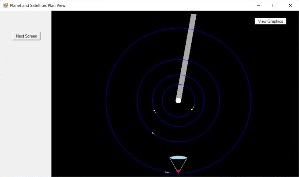
To obtain graphical displays, a button “Planet and Satellites View” is clicked.
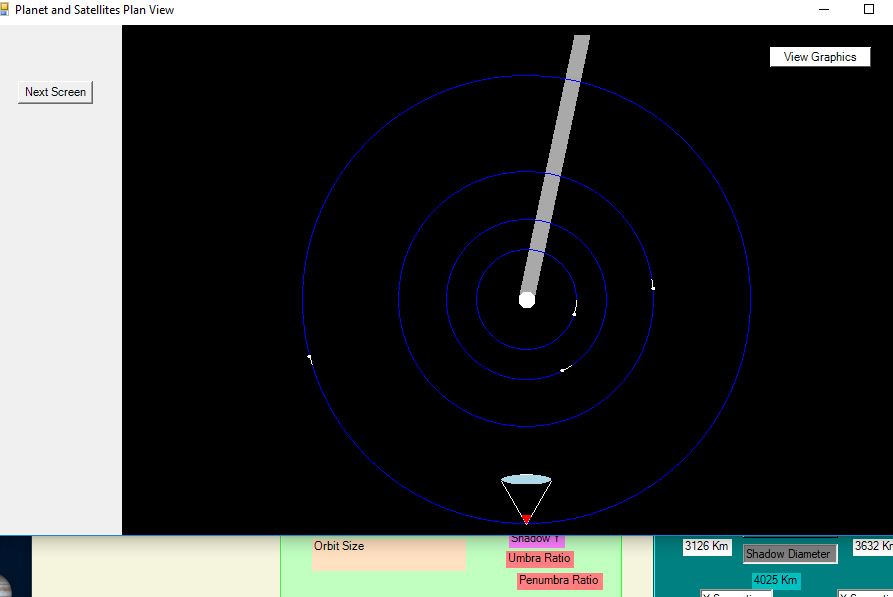
Planet and Satellites view
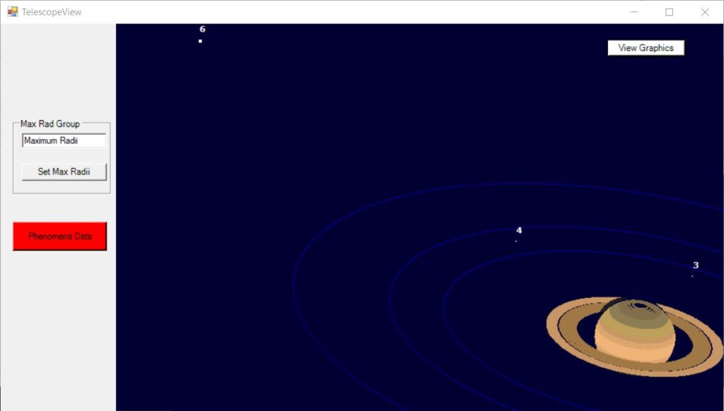
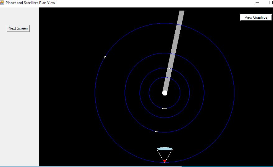
The button “View Graphics” shows a Plan view of the system, looking down on the north pole, such that they revolve counter-clockwise. The satellite orbits are shown to scale.
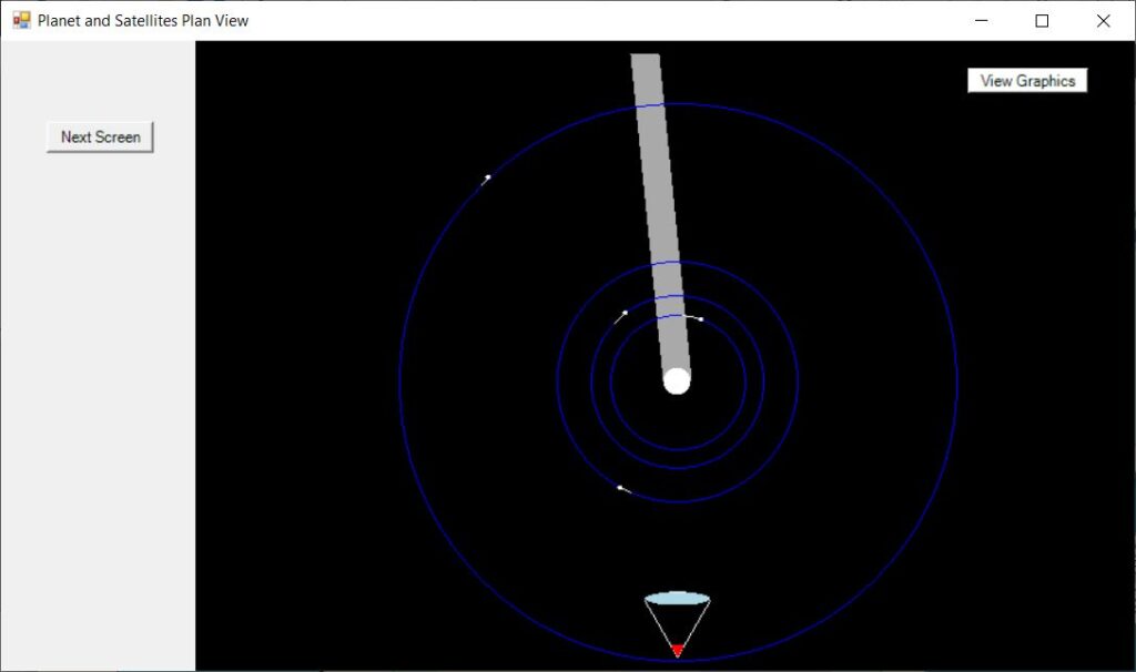
Note that, in this case, only Tethys, Dion, Rhea, and Titan are shown because the others are too dull to see with the chosen aperture.
The position of the observer is represented by a symbolic eye and the direction of the shadow cast by the planet is shown in order to help with seeing possible eclipses and shadows (more important for Jupiter).
A line is drawn from the planet in the direction of travel showing the movement in 2 hours. This gives an idea of when at a later time, or an earlier time, interesting phenomena may occur.
To see a representation of the view through the telescope, the “Next Screen” button is clicked, followed by “View Graphics“. This then displays the planet, the satellites, and a faint path showing roughly the orbit of the satellite.
Only satellites which are brighter than a limiting magnitude are shown.
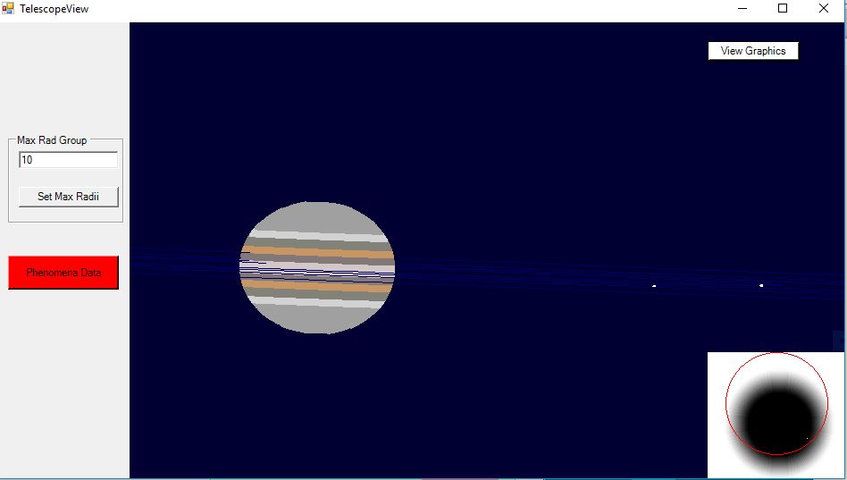
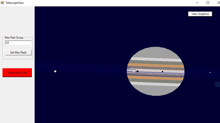
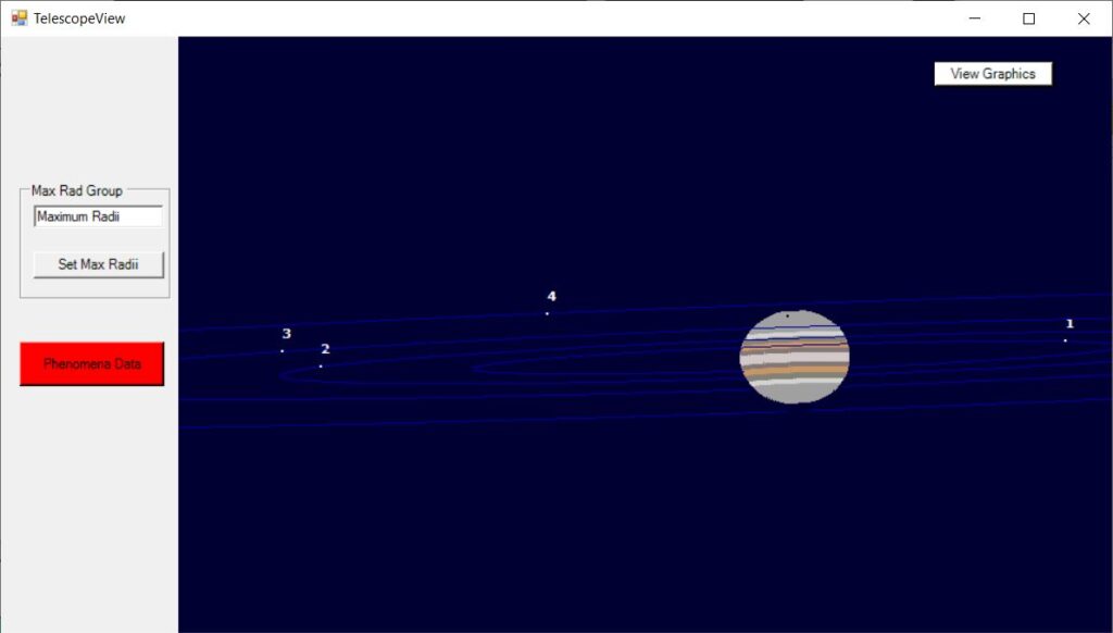
Telescope view
This limiting magnitude can be made to depend on the aperture of the telescope. It is assumed that an 8 inch aperture has a limiting visual magnitude of 11.0 and other apertures scale the value accordingly. Currently, no allowance is made for the effect of a photographic time exposure. The telescope aperture can be chosen in the main form, discussed above.
For the Jovian satellites, the sizes of the planet and satellites are drawn to scale, provided the scale is large enough to show the satellites correctly.
For Saturn, the number of pixels displayed is designed to correspond to the intensities, except for Titan, which is shown to scale if possible.
The scale of the whole image can be altered by setting the number of planetary radii to be displayed. Thus, a small value will cause the planet to take up a large area on the screen and so allow the satellite system and the “surface” of the planet to be scaled up appropriately. The value chosen will depend on how much of the satellite system the user desires to see – usually one first uses the default value, which fits the whole system optimally on the screen, and then chooses a small value in order to zoom in. If there are any satellite phenomena occurring, the zoom will not be so great as to omit those satellites involved. It is suggested that between 5 and 10 be used for Jupiter and between 10 and 20 for Saturn.
If a satellite is eclipsed by the planet, it is still shown, but in a dull grey to indicate that it is not visible. If a satellite is occulted, it is not shown. If a shadow is thrown onto the planet, the position of the shadow is shown as a filled black circle. See Jupiter examples below.
The planet itself is shown with bands of color at different latitudes. If the user has access to the source code, he or she may wish to modify the actual colors.
If the phase is significantly less than one (really only possible for Mars, with a slight effect for Jupiter), this is shown by not drawing the planet beyond the terminator.
The limiting latitudes for the polar caps of Mars are estimated, and displayed as white. The rest of Mars is shown as varying ocher color.
In the rare case that a mutual satellite phenomenon occurs, a graphical representation appears in the bottom right-hand corner of this screen. It shows the shadow, with umbra surrounded by penumbra and the outline of the eclipsed satellite in red. The intensity of the penumbra varies from black to white in the correct manner from the inside to the outside.
In order to find out more about any satellite phenomena (not including mutual phenomena or shadows) which may be occurring, the user can click the Phenomena Data button which appears on the graphics screen.
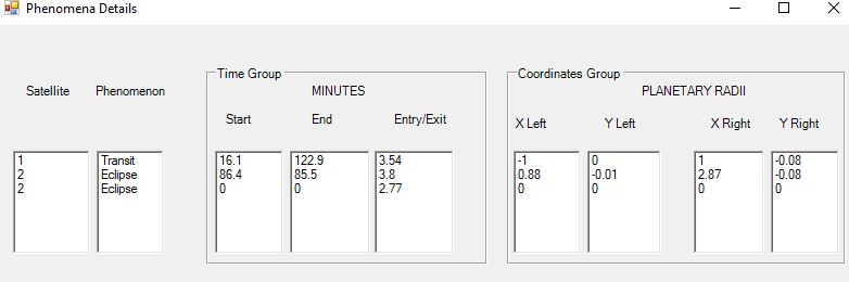
Phenomena Data form
This will give, for any phenomenon except a shadow (information on position and size of a shadow can be obtained by using the “Satellite Details” button mentioned above):
The minutes since it began; the minutes until it finishes; the minutes it takes to enter or exit (cross the planet surface or the edge of the umbra of the shadow in the case of an eclipse); on a second line, the minutes to cross the penumbra in the case of an eclipse; the X and Y coordinates (in terms of planetary radii) of the left-hand end and the right-hand end of it.
It is thus possible to estimate when and where to look for the faint reappearance after an eclipse and what new times to enter into the program to check for the events.
See examples below under Eclipse and shadows for an example of this screen.
Note:
When running the program, it is sometimes useful to delete all forms except the Main form and then change date or time and proceed from that point. This often allows the user to try several different times without restarting the program. However, this can sometimes produce spurious results, at which time it is recommended that the program be stopped and then restarted.
Accessing and Using SatGraph
Click on the files mentioned below and save them in a folder e.g.”Satgraph files from web” . This includes the data files and the executable file.
(These files need to be in “.bin”
Unfortunately, I am having trouble obtaining the Visual Basic solution file or the executable file for the user to use. I am working on it to try to do so. WordPress says the .exe file is “not permitted for security reasons”. If you contact me by email, I will try to get an executable copy of the program to you.
The text files are here (see below) and may be of interest.
You may find it useful to look at the contents of these data files.
NOTE: The program has recently been changed to use to VSOP87 theory for the planetary positions. See, for example, MEEUS II, Chapter 31 and Appendix 2 or
https://github.com/ctdk/VSOP87/blob/master/VSOP87D.xxx where xxx is Mer, Ven, Ear, Mar, Jup, Sat, Ura, or Nep.
More will be said about this elsewhere.
Files read by the program
- Plan2000II.txt
This file contains information about each of the planets, Mercury to Neptune (including Earth). Plan2000II contains slightly-changed data following MeeusII and ESII. (see the references)
- 8 VSOP87D files.
- Sat2000III.txt
This file contains information about the satellites Phobos, Deimos, Io, Europa, Ganymede, Callisto, Mimas, Enceladus, Tethys, Dione, Rhea, Titan, Hyperion, and Iapetus. The data are the same as for the planets, except that the planet data include inclination and Longitude of Ascending node of the equator.
- The files Jovian _Periodic_Coeffs.txt and Jovian_Periodic_Formulae.txt contain data from Chapter 43 of Meeus II for obtaining high accuracy for the positions of the satellites of Jupiter. The method is based on the theory due to:
J.H. Lieske, Astronomy and Astrophysics, Vol 82, pp340-348 (1980), and
J.H. Lieske, Astronomy and Astrophysics, Vol 176, pp146-158 (1987).
More information on the content of these files is given in the “Programming Details” section.
If you do not have Visual Basic, you can run the executable program as follows:
Click on and Save the executable file “WindowsApplication1_0.exe” in the folder which contains the 12 data files.
Run the executable file.
However, if you do have Visual Basic, you should be able to get the source code (NOTE: I am still working on this to allow the reader to view and/or modify the code)
This enables you to modify it or to investigate the code for a better understanding of the calculations involved.
In this case, double click WindowsApplication1.sln VB users will then be able to use Solution Explorer to obtain the Designer and source code and start the program by “start debugging”. It is really necessary to have access to the source code if this website is to be truly useful in explaining Satgraph.
Interesting Examples
The satellite system of Jupiter (“Jovian” or “Galilean” satellites) provides the most interest so three such examples are given:
(i) Mutual eclipse,
(ii) Eclipses and shadows, and
(iii)Galileo’s view in January 1613.
Modern astronomy magazines often give predictions for mutual occultations and eclipses of the satellites – often presented by Jean Meeus, e.g. Sky and Telescope December 2002, pp. 100-103. Here, I refer to an older reference, that of Bertrand Peek in “The Planet Jupiter”. On p.219, he gives an account of Ganymede eclipsing Io. Satgraph gives the maximum coverage at UT 02:21:30 on 9th February 1920.
(i) Mutual Eclipse
Here are some images of the computer screen for this date and time.
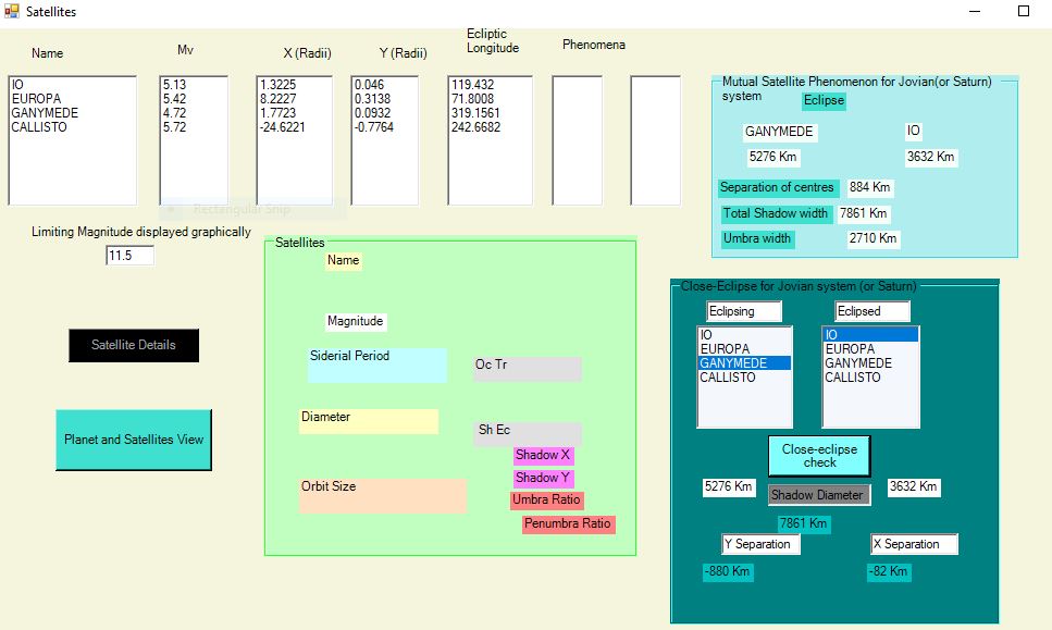
In order to get extra details, Ganymede and Io have been selected in the “close-eclipse” box as shown.


Here is another example from 23 May 1926, UT03:54:0
Reference is made to this event in “The Planet Jupiter”, by Bertrand M Peek, page 219.
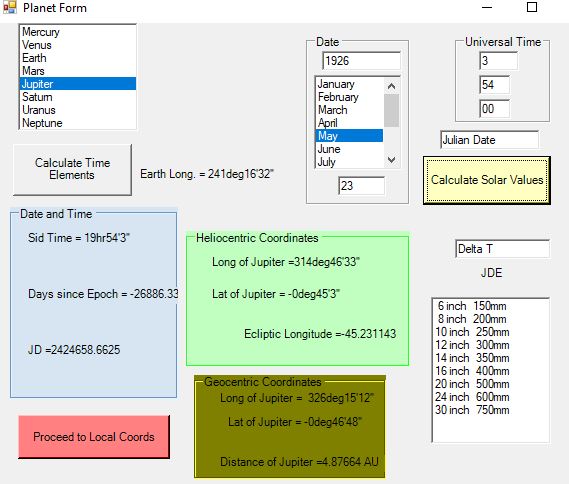
It is useful to enter the mid-times given by Meeus in the above reference, along with ΔT = 64 seconds, for the mutual eclipses listed by him.
In particular, the plan of the satellite system and the diagram of the shadow superimposed on the eclipsed satellite are very helpful in understanding the eclipse.
(ii) Eclipses and shadows
I shall give more-modern references, but here is another interesting example from 1926 – 21 May, 1926 at UT = 00:00:00.
Io is in transit and has a shadow, Europa is in eclipse, and Ganymede has a shadow.
The Telescope View screen shows the size and position of the shadow of Ganymede, as well as the transit and shadow of Io.
This screen uses maximum Jupiter radius of 10 in order to make Jupiter appear larger.
The following screen gives information about the satellite phenomena occurring.
(iii) Galileo’s sighting of Neptune
Refer to Scientific American, December 1980, p52 Galileo’s Sighting of Neptune by Stillman Drake and Charles T. Kowal .
Or http://www.dioi.org/vols/wf0.pdf for article by Charles T Kowal
or http://eotvos.dm.unipi.it/galileo%20neptune%20SAit%202009.pdf by Anna M Nobili
The time and date I show here is 06 January 1613, UT = 05:37:00 . His chart is at the bottom left of p.53 of Scientific American or on pages 14 and 15 Fig. 4) of Nobili.
Satgraph shows what Galileo “saw” of the satellite system, if allowance is made for the shortcomings of his telescope (e.g. his surface of Jupiter is fuzzy and blown up by a factor of about 1.1 so his estimates of distance in Jovian radii need to be multiplied by 1.1).
The articles are to show where he saw what we now know to be Neptune.
When Satgraph is used to find the position of Neptune at UT=05:37, it gives a separation of the two planets of about 241″, or 12.3 Jovian radii. This compares with Io at 4.77 Jovian radii. The assertions of Drake and Kowal and, even more so of Nobili, are approximately verified.
SatGraph calculates, for Jupiter, among other things
RA = 11h49m23s Declination = 2o 37′ 12″,
Altitude= 42deg11’37”, Azimuth=214deg4’8″
and produces the screens shown above.
SatGraph (see the screen above) calculates that the satellites , from left to right (numbers are multiples of Jupiter’s radius), are at:
Ganymede (shown with 2 dots by Galileo) -9.37 (-8.5 for Galileo)
Europa (shown with 1 dot ) -8.65 (-7.9)
Callisto (shown with 3 dots ) -4.53 (-4.1)
Io (no dots ) +4.92 (+4.5)
The numbers in brackets would be Galileo’s estimates, which are seen to agree closely. SatGraph also shows that Callisto is throwing a shadow on the very top left-hand corner of Jupiter (I can’t help thinking that Galileo deserved to have a telescope that was good enough to show the shadow – he would have been enthralled).
It is on this chart that Drake and Kowal, and Nobili believe that Galileo saw Neptune but rubbed it out. They have placed it at about 1.8 times the distance of Io and slightly below the plane.