This is an inexpensively-built spectrograph for insertion into the focussing tube of a moderately-sized (amateur’s) telescope to give quality spectra of stars and nebulae.
The best website I have found for this is http://www.astrosurf.org/buil/us/stage/calcul/design_us.htm, “Theoretical Parameters for the Design of a Classical Spectrograph”.
Based on the terminology used in the above site, the specifications of the MRS135 are:
Spectrograph Construction
- f1 = 135mm
- f2 = 51mm
- m = 1200 lines/mm
- Grating size is 50mm square
- γ = 42 degrees
- X = 100mm
- Camera lens F# = 2
- Detector is Canon EOS350D , pixel size 6.42microns square, maximum 3456 pixels in plane of dispersion
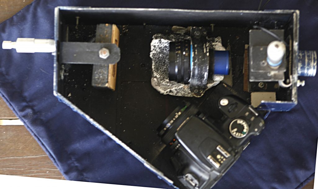
My second version of the spectrograph has been built from aluminium sheeting (not wood) .
I have set the diffraction grating into a wooden frame. (It may be possible to purchase a grating holder but this can be expensive.)
It is important for the axis of rotation to go through the face of the grating, so it has a rod above, attached to a strut, and another rod below and passing through the floor. Rotation is done using a micrometer through the rear wall. This allows the desired wavelength to be “dialled up” approximately before locating the star. It does not, however, give a precise wavelength and estimation from the spectral image is still required.
Rotation of the diffraction grating is such that positive or negative spectral orders can be used, at least up to second order on one side. Of course, zero order can also be used for finding and focusing the star without dispersion.
The input tube is the tube from a 1.25” eyepiece, and it has been firmly attached onto the input face. In order to reduce flexing when the MRS135 is attached to the focusing tube, the base and the input plate are made of thicker aluminium than the sides and top.
Often it is used without a slit (see later), but simple slits can be made by removing the filter glass from a 1.25” filter, replacing it with bits of 2 razor blades epoxied close together, and the filter assembly screwed into the end of the eyepiece tube. Of course this then has to be placed close to the infinity focal point of the collimating lens. Slits are other items which can be purchased. However, as with grating holders, they are not cheap and their mounting in the correct position would have to be considered. Certainly a good slit which was adjustable from, say, 20 microns up to 100 microns would be very useful. The latest model has been made with a slit mechanism ( shown in the image below) with micrometer adjustment but this can be removed for stars.
The 135mm collimating lens can be seen in the image.
The Canon EOS350D, with 50mm lens, can also be seen.
Discussion of the Mathematics in the website
Step 1
It is unlikely that there will be vignetting at the collimator because of the high F numbers of telescopes compared with camera lenses. My telescopes are F/6 (Newtonian), F/5 (Newtonian) and F/4 (Schmidt Newtonian).
Step 2
I usually use the F/4 SN10 telescope for spectroscopy so the diameter of the exit beam at the collimator is 135⁄4 = 34 mm.
Step 3
This contains a very important formula for calculating the angles α and β, given the central wavelength, λ0 of the spectrum.
Note: Sin(α) + Sin(α-γ) = 2Sin(α-γ/2).Cos(γ/2)
So Sin(α-γ/2) = k.m.λ0/(2.Cos(γ/2)) or Sin(β+γ/2) = k.m.λ0/(2.Cos(γ/2)), where order k can be positive or negative.
Alternatively, if it was angle α of the diffraction grating that was known, then the central wavelength could be found.
Step 4
The minimum grating dimension is the value calculated in Step 2 divided by Cos(α). This can become large, when α is large, and so it is desirable to have a larger grating than the 30mm one suggested in the website.
Step 5
For a given image, α is fixed and we have Sin(α) + Sin(β) = k.m.λ
Differentiation gives dβ/dλ = k.m/Cos(β)
i.e. dλ/dβ = 107 Cos(β)/(k.m) A/radian, where A represents Angstroms, one Angstrom being 10-10m or 0.1Nm. This gives the rate of change of wavelength with respect to the angle β but we want it with respect to the linear distance across the detector, which we will call s.
Then dλ/ds = 107Cos(β)/(k.m.f2) A/mm. This is called the Reciprocal Linear Dispersion. Alternatively, if we specify the width of a pixel as p microns, and denote the dispersion per pixel by ρ, we have
ρ = 104.p.Cos(β)/(k.m.f2) A/pixel
Step 6
For my configuration, I could not safely reduce X to less than 100mm. Also, with using the EOS350D as the detector, N (or p.N which is the ‘length’ of the detector) is very large and, consequently, the second term in the calculation of d2 is very large. Hence, there is no way of avoiding vignetting of the CCD. I will show the calculations appropriate for the MRS135 in a later section. In practice, I can get a maximum of 2000 pixels included in the spectrum and this has severe vignetting, and hence attenuation of the signal, at the edges.
Hence, the extreme wavelength limits, calculated in Step 7, are not relevant to the MRS135.
Step 8
I find the formulae given in this section somewhat confusing and will attempt to derive them in a more-logical way.
First, we find the Full Width at Half Maximum, FWHMt, of the image of the star on the detector. This depends on the optics and the configuration of the spectroscope and also the size of the star at the entrance. This latter is f.φ where f is the focal length of the telescope and φ is the astronomical seeing (in radians). For example, if φ is 3 seconds of arc, its value in radians is 3/(180/Pi*3600) = 3⁄206265 = 1.45*10-5 and if f=1000mm, then the size of the star at the entrance of the spectrograph is 1.45 *10-2 mm = 14.5 microns.
It is desirable to keep the image of the star (or of the slit if there is one) as small as possible as it passes through the spectrograph, since the resolution obviously cannot be smaller than this size (the FWHMt).
In fact, dλ = FWHMt*Dispersion/mm
= FWHMt*Cos(β)/(k.m.f2)
Note that the expression r.(Tan( α) + Sin(β)/Cos(α)) in Step 8, where r is the anamorphic factor Cos(α)/Cos(β), can be simplified thus:
r.(Tan( α) + Sin(β)/Cos(α)) = Sin(α)/Cos(β) + Sin(β)/Cos(β) = (Sin(α) + Sin(β))/Cos(β)
= k.m.λ /Cos(β)
So the expression for R, the resolving power of the spectrograph, given in the website can equivalently be expressed as R = (f2/FWHMt)*k.m.λ /Cos(β). [This can also be derived by dividing λ by the expression for dλ derived above.]
This is a more-useful way of expressing R since it gives good clues as to what can be changed to increase R, the resolving power.
See the example given below.
It remains to discuss the important expression given for calculating FWHMt. It uses FWHMc and FWHMo which are the full width at half maximum of the image of a point source produced by the collimating lens and the camera lens respectively. The website states that for standard photographic lenses typical values are FWHMc = 10 microns (.01mm) and FWHMo = 15 microns (.015mm).
Then (FWHMt) ² = (r.f2/f1) ² × (φ ² .f ² + FWHMc ² ) + FWHMo ² + p ² . The first term on the right hand side is large and it can be reduced by making f2/f1 small, that is by making the focal length of the collimating lens greater than that of the camera lens, in effect causing a demagnification of the image. This is the reason that I chose 135mm for the collimating lens, even though it added a little to the size of the spectrograph.
For the size of the star image of 14.5 microns calculated above and taking r = 1 as an approximation, this gives, for the MRS135,
(FWHMt) ² = 0.3702.*310.25 + 225 + 6.422 = 308.7, giving FWHMt = 18 microns. This is approximately 3 pixels on the detector.
Example
(a) Consider a central wavelength λ0 = 5500A (550Nm) and spectral order k = -1.
To find α, the expression on the right hand side in Step 3 needs to be multiplied by 10^-7 because of the units used.
Also, Cos(γ/2) = 0.9483
α-γ/2 = -20.364 degrees
α = -1.864 deg.
β = -38.864 deg.
L= 33.8mm
r = 1.284
From Step 5, Dispersion ρ = 104p.Cos(β)/(k.m.f2) A/pixel = -0.83 A/pixel
f.φ = 14.54 microns
FWHMt = 18.35 microns = 2.85 pixels
To find dλ, using the values in the units used, the expression in Step 8 needs to be multiplied by 104, giving
dλ = -2.38 Angstroms and R = -2310
(b) It is feasible with the MRS135 to use spectral order -2 and the results with this and the same central wavelength are:
α = -25.6 deg. β = -62.6 deg. r = 1.96 ρ = -0.25A/pixel
FWHMt = 20.75 microns = 3.23 pixels
dλ = -0.80 Angstroms and R = -6914
Here is a simple Excel spreadsheet which performs the above calculations
Different values of the spectral order and the central wavelength can be inserted in it. If you have designed a spectrograph with different specifications, you can also try those values.
Vignetting at the Detector
It has been pointed out above that with the high value of X and the potentially large span of the CMOS detector in the EOS350D, it is not possible to cover the whole of the detector or to avoid some vignetting (i.e. loss of light) at the edges of the image.
I have done some calculations which give approximate values for the number of pixels on the detector which have:
- All light received
- At least half the light received
- At least some light received.
These are approximate because they do not allow for the circularity of the camera lens.
If D2 is the diameter of the camera lens (assumed to be 25mm), we have
- Dall = (f2/X)*(D2-d1/r)
- Dhalf =(f2/X)*D2
- Dnone = (f2/X)*(D2+d1/r)
For Example (a) above, these values are:
- Dall = 0 i.e. none of the detector receives all the light
- Dhalf = 12.5 mm = 1986 pixels receive at least half the light
- Dnone = 25.6mm i.e. all of the detector receives some light
For Example (b), the corresponding values are:
618 pixels; 1986 pixels; and 3354 pixels.
↑¹²³αβγ¼½¾×
Comments
- It can be seen from the previous section that the camera lens should have a large aperture.
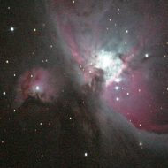
- A crude slit has been used and is needed for testing with lamps, e.g. Neon or Mercury, and has been used to obtain the spectrum of M42, the Orion nebula. Nevertheless, a better slit would be desirable. I have attempted to add a reference spectrum but the slit needs to be narrow, and the reference light (probably via an optical fiber) needs to be positioned on the slit. Of course, the image of the star needs to be positioned on the slit and this is difficult as the star can’t be seen at the same time unless some beam splitting is employed. Best results have been obtained without a slit, which is very acceptable for stellar spectra.
- A variation of the spectrograph has been made with a 50mm collimating lens (called the MRS50). It is slightly more compact (and puts less strain on the telescope) but the reduction in the size of the image obtained by using the longer focal length lens in the MRS135 has given me better results.
- One drawback with using an EOS350D (or any DSLR) as the detector is the lack of response in the Ultra Violet and in the Infra Red. Accordingly, I have recently purchased a second (used) EOS350D and removed the IR blocking filter. These cameras are now cheap enough to justify this. However, removal of the filter is not trivial and to have it done professionally probably costs more than the used camera. The results that I am obtaining are, however, very encouraging. Whereas the spectral range with the unmodified camera was about from 4200 Angstroms (420Nm) to 6800A, the range now is about 3900A to perhaps 10000A.
References
http://astrosurf.com/buil/us/spe2/hresol.htm
h
Practical Amateur Spectroscopy , Stephen F. Tonkin (Ed.) , 2002 , Springer